Create a complete variability for a collection of spatial interaction models

This function represents graphically the variability of the flows represented by the spatial interaction models contained in a collection (a sim_list object).

Usage

# S3 method for class 'sim_list'
autoplot(
  object,
  flows = c("full", "destination", "attractiveness"),
  with_names = FALSE,
  with_positions = FALSE,
  cut_off = 100 * .Machine$double.eps^0.5,
  adjust_limits = FALSE,
  with_labels = FALSE,
  qmin = 0.05,
  qmax = 0.95,
  normalisation = c("origin", "full", "none"),
  ...
)

Arguments

object: a collection of spatial interaction models, a sim_list
flows: "full" (default), "destination" or "attractiveness", see details.
with_names: specifies whether the graphical representation includes location names (FALSE by default)
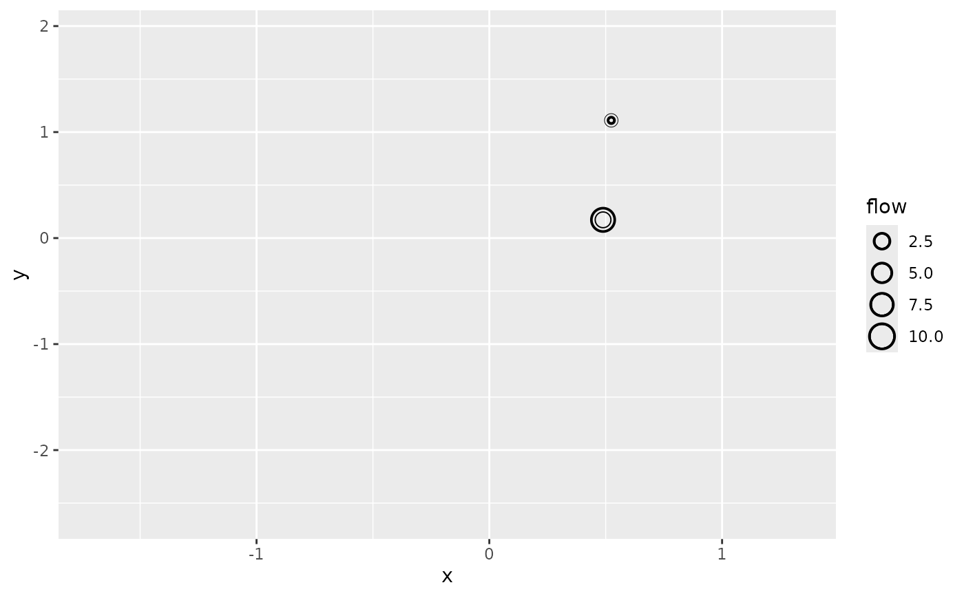
with_positions: specifies whether the graphical representation is based on location positions (FALSE by default)
cut_off: cut off limit for inclusion of a graphical primitive when with_positions = TRUE. In the attractiveness or destination representation, circles are removed when the corresponding upper quantile value is below the cut off.
adjust_limits: if FALSE (default value), the limits of the position based graph are not adjusted after removing graphical primitives. This eases comparison between graphical representations with different cut off value. If TRUE, limits are adjusted to the data using the standard ggplot2 behaviour.
with_labels: if FALSE (default value) names are displayed using plain texts. If TRUE, names are shown using labels.
qmin: lower quantile, see details (default: 0.05)
qmax: upper quantile, see details (default: 0.95)
normalisation: when flows="full", the flows can be reported without normalisation (normalisation="none") or they can be normalised, either to sum to one for each origin location (normalisation="origin", the default value) or to sum to one globally (normalisation="full").
...: additional parameters, not used currently

Value

a ggplot object

Details

The graphical representation depends on the values of flows and with_positions. It is based on the data frame representation produced by fortify.sim_list(). In all cases, the variations of the flows are represented via quantiles of their distribution over the collection of models. For instance, when flows is "destination", the function computes the quantiles of the incoming flows observed in the collection at each destination. We consider three quantiles:

a lower quantile qmin defaulting to 0.05;
the median;
a upper quantile qmax defaulting to 0.95.

If with_position is FALSE (default value), the graphical representations are "abstract". Depending on flows we have the following representations:

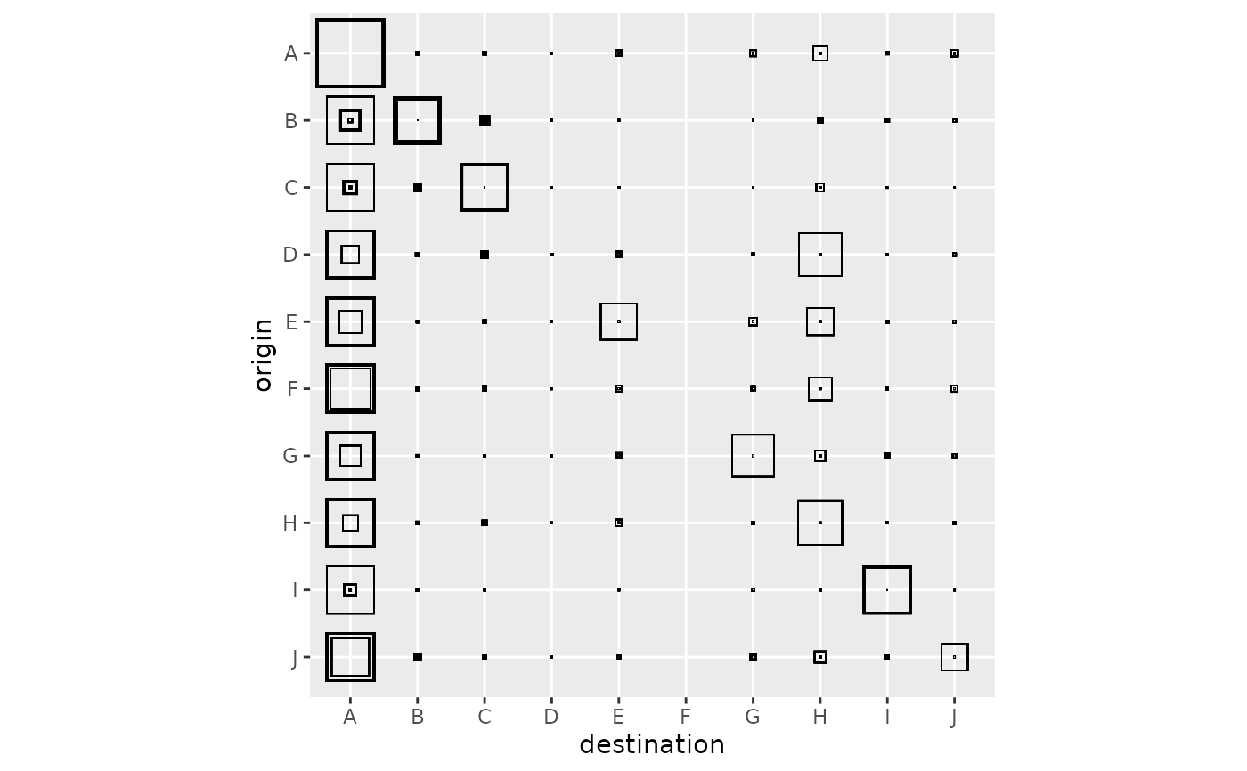
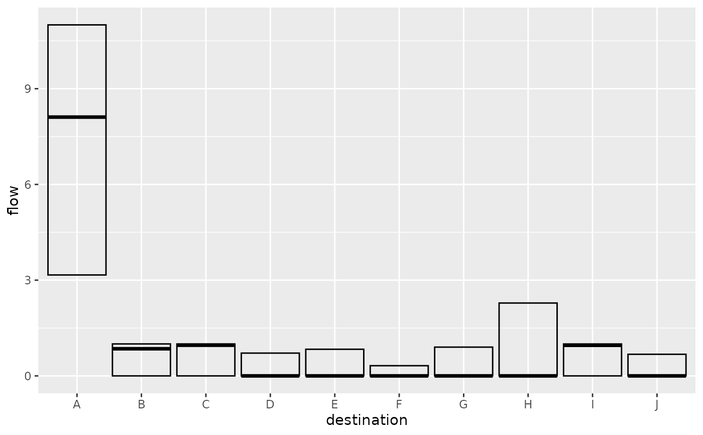
"full": the function displays the quantiles over the collection of models of the flows using nested squares (flows()). The graph is organised as matrix with origin locations on rows and destination locations on columns. At each row and column intersection, three nested squares represent respectively the lower quantile, the median and the upper quantile of the distribution of the flows between the corresponding origin and destination locations over the collection of models. The median square borders are thicker than the other two squares. The area of each square is proportional to the represented value.
"destination": the function displays the quantiles over the collection of models of the incoming flows for each destination location (using destination_flow()). Quantiles are represented using ggplot2::geom_crossbar(): each location is represented by a rectangle that spans from its lower quantile to its upper quantile. An intermediate thicker bar represents the median quantile.
"attractiveness": the function displays the quantiles over the collection of models of the attractiveness of each destination location (as given by attractiveness()). The graphical representation is the same as for "destination". This is interesting for dynamic models where those values are updated during the iterations (see blvim() for details). When the calculation has converged (see sim_converged()), both "destination" and "attractiveness" graphics should be almost identical.

When the with_names parameter is TRUE, the location names (location_names()) are used to label the axis of the graphical representation. If names are not specified, they are replaced by indexes.

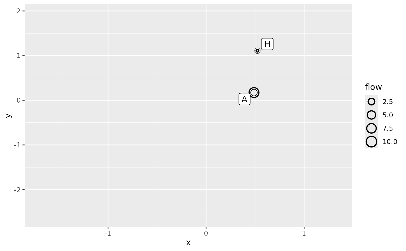
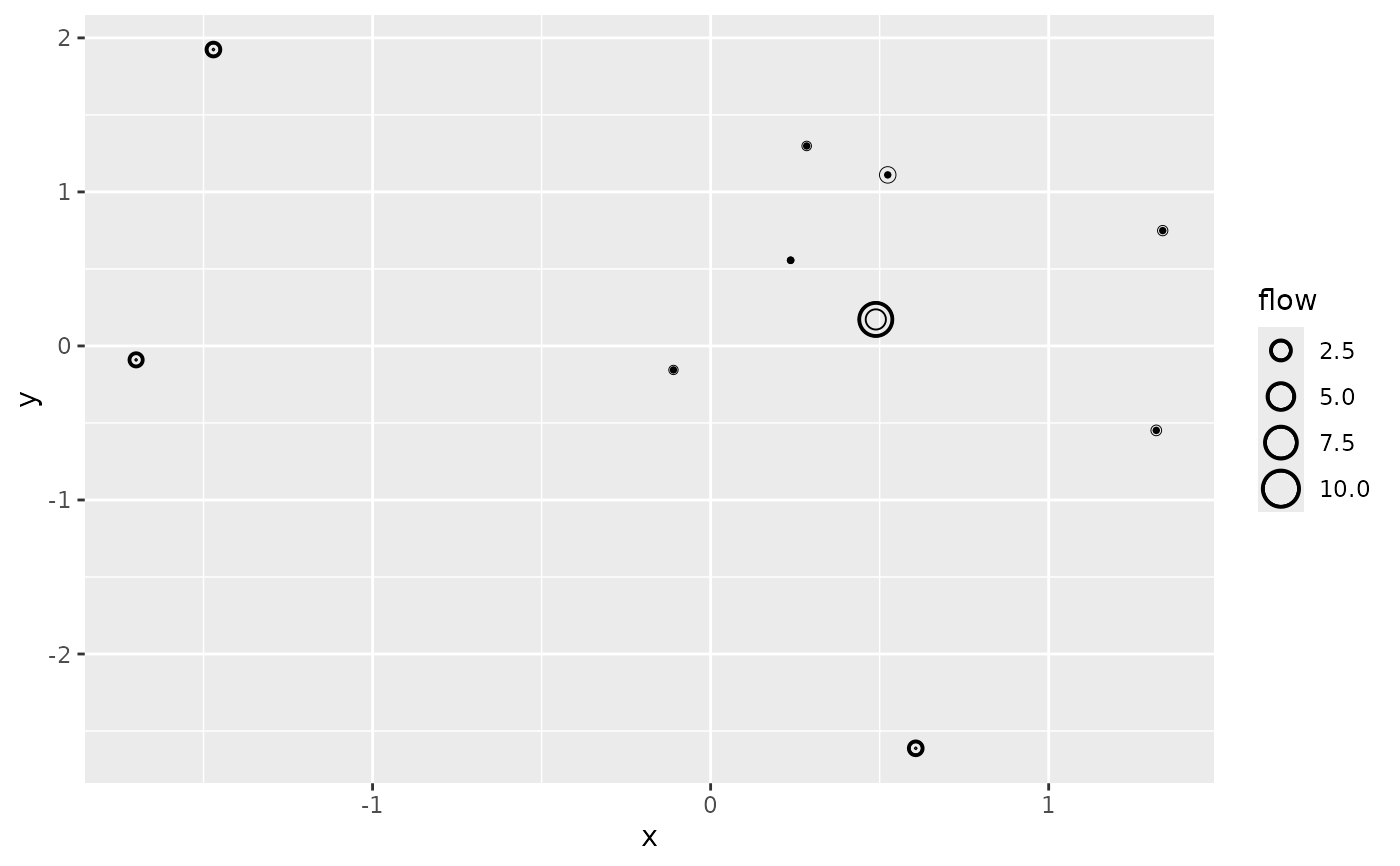
When the with_positions parameter is TRUE, the location positions (location_positions()) are used to produce more "geographically informed" representations. Notice that if no positions are known for the locations, the use of with_positions = TRUE is an error. Moreover, flows = "full" is not supported: the function will issue a warning and revert to the position free representation if this value is used.

The representations for flows="destination" and flows="attractiveness" are based on the same principle. Each destination location is represented by a collection of three nested circles centred on the corresponding location position, representing respectively the lower quantile, the median and the upper quantile of the incoming flows or of the attractivenesses. The diameters of the circles are proportional to the quantities they represent. The border ot the median circle is thicker than the ones of the other circles.

When both with_positions and with_names are TRUE, the names of the destinations are added to the graphical representation. If with_labels is TRUE the names are represented as labels instead of plain texts (see ggplot2::geom_label()). If the ggrepel package is installed, its functions are used instead of ggplot2 native functions.

Examples

positions <- matrix(rnorm(10 * 2), ncol = 2)
distances <- as.matrix(dist(positions))
production <- c(2, rep(1, 9))
attractiveness <- c(2, rep(1, 9))
all_flows <- grid_blvim(distances, production, seq(1.05, 1.45, by = 0.1),
  seq(1, 3, by = 0.5),
  attractiveness,
  bipartite = FALSE,
  epsilon = 0.1, iter_max = 1000,
  destination_data = list(names = LETTERS[1:10], positions = positions),
  origin_data = list(names = LETTERS[1:10], positions = positions),
)
ggplot2::autoplot(all_flows, with_names = TRUE)

ggplot2::autoplot(all_flows, with_names = TRUE, normalisation = "none")

ggplot2::autoplot(all_flows,
  flow = "destination", with_names = TRUE,
  qmin = 0, qmax = 1
)

ggplot2::autoplot(all_flows,
  flow = "destination", with_positions = TRUE,
  qmin = 0, qmax = 1
) + ggplot2::scale_size_continuous(range = c(0, 6))

ggplot2::autoplot(all_flows,
  flow = "destination", with_positions = TRUE,
  qmin = 0, qmax = 1,
  cut_off = 1.1
)

ggplot2::autoplot(all_flows,
  flow = "destination", with_positions = TRUE,
  with_names = TRUE,
  with_labels = TRUE,
  qmin = 0, qmax = 1,
  cut_off = 1.1
)