Return the iteration history of the algorithm used to build a spatial interaction model
Source:R/sim.R
sim_history.RdSome spatial interaction models are the result of an iterative calculation,
see for instance blvim(). This function returns the history of the
iterations of this calculation when it has been recorded, and NULL when
this is not the case, in particular when the spatial interaction model is
not the result of an iterative calculation. The function applies also to a
collection of spatial interaction models as represented by a sim_list.
Value
a data frame of class blvim_history describing the iterations of
the algorithm, or NULL if no history was recorded, as described above.
Use summary.blvim_history() and autoplot.blvim_history() to describe
and display it. In the case of a
sim_list the function returns a single data frame gathering the
histories of all models (see grid_sim_history()), or NULL if no
history was recorded for any of them.
Details
Currently, only the gradient algorithms of blvim() can record their
iteration history, when asked to do so with the history parameter of
blvim_gradient_control(). For all other spatial interaction models, the
function returns NULL.
The history is a data frame with one row per iteration, including the initial point (iteration 0) and the final one, and the following columns:
iteration: iteration number;gap: duality gap at the current point;potential: potential at the current point (seesim_potential());step: accepted step in the line search (0 for the final point);step_norm: Euclidean norm of the accepted step in the rescaled attractivenesses (0 for the final point);line_search_reductions: number of step reductions in the line search;n_active: number of active destinations (with a positive rescaled attractiveness) at the current point, which changes when the algorithm moves from one face of the simplex to another;min_U: smallest rescaled attractiveness at the current point.
When multiple starting points are used in blvim(), the history is
available only for the retained models, that is the selected one and, if
keep_runs = TRUE, the ones returned by sim_runs().
Applied to a sim_list, the function returns the histories of all its
models in a single data frame; see grid_sim_history().
Examples
distances <- french_cities_distances[1:10, 1:10] / 1000 ## convert to km
production <- log(french_cities$population[1:10])
attractiveness <- log(french_cities$area[1:10])
model <- static_blvim(distances, production, 1.5, 1 / 100, attractiveness)
sim_history(model) ## must be NULL
#> NULL
model <- blvim(distances, production, 1.5, 1 / 100, attractiveness,
  algorithm = "gradient",
  control = blvim_gradient_control(history = TRUE)
)
sim_diagnostic(model)
#> BLV model obtained with the "gradient" algorithm.
#> ℹ The algorithm converged after 35 iterations:
#> • Number of potential evaluations: 52.
#> • Duality gap: 5.063753e-05.
#> • Return status: "converged".
#> • Iteration history (35 rows) available via `sim_history()`.
history <- sim_history(model)
head(history)
#>   iteration       gap potential        step  step_norm line_search_reductions
#> 1         0 13.202832  217.7197 0.001953125 0.03413314                      8
#> 2         1  6.812050  217.9130 0.001953125 0.02952523                      0
#> 3         2 12.405944  217.9645 0.001220703 0.02360967                      1
#> 4         3  6.530400  218.1298 0.001220703 0.01457876                      0
#> 5         4  5.428017  218.2434 0.001525879 0.01524895                      0
#> 6         5  7.344117  218.3899 0.001907349 0.02264912                      0
#>   n_active      min_U
#> 1       10 0.09413106
#> 2       10 0.08603530
#> 3       10 0.07773592
#> 4       10 0.08089690
#> 5       10 0.07543261
#> 6       10 0.06521078
summary(history)
#>
#> ── Iteration history of a gradient ascent ──
#>
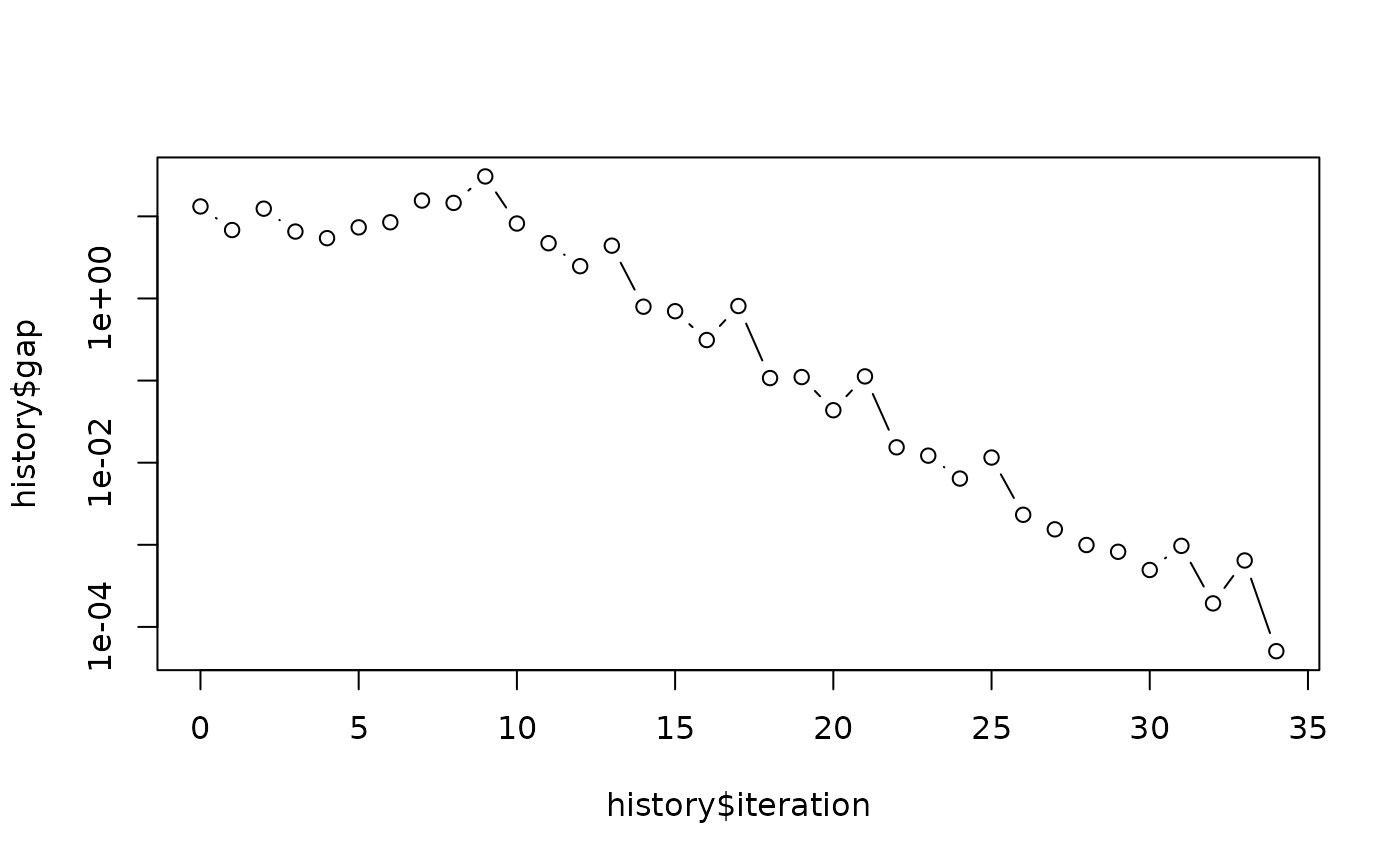
#> • 35 iterations, potential from 217.7197 to 225.1725.
#> • Final duality gap: 5.064e-05.
#> • Convergence rate of the duality gap: 0.6415 per iteration.
#> • Line search: 17 step reductions, smallest accepted step 0.00101.
#> • Active destinations: from 10 to 8, 2 face changes, the last one at iteration
#> 9.
#> • The final configuration is on a face of the simplex.
plot(history$iteration, history$gap, log = "y", type = "b")