Create a complete variability plot for spatial interaction models in a data frame

This function combines variability representations of spatial interaction models similar to the ones produced by autoplot.sim_list() into a single ggplot. It provides an alternative graphical representation to the ones produced by autoplot.sim_df() and by grid_autoplot() for collections of spatial interaction models in a sim_df object.

Usage

grid_var_autoplot(
  sim_df,
  key,
  flows = c("full", "destination", "attractiveness"),
  with_names = FALSE,
  with_positions = FALSE,
  cut_off = 100 * .Machine$double.eps^0.5,
  adjust_limits = FALSE,
  with_labels = FALSE,
  qmin = 0.05,
  qmax = 0.95,
  normalisation = c("origin", "full", "none"),
  fw_params = NULL,
  ...
)

Arguments

sim_df: a data frame of spatial interaction models, an object of class sim_df
key: the wrapping variable which acts as a group identifier for spatial interaction models
flows: "full" (default), "destination" or "attractiveness", see details.
with_names: specifies whether the graphical representation includes location names (FALSE by default)
with_positions: specifies whether the graphical representation is based on location positions (FALSE by default)
cut_off: cut-off limit for inclusion of a graphical primitive when with_positions = TRUE. In the attractiveness or destination representation, circles are removed when the corresponding upper quantile value is below the cut-off.
adjust_limits: if FALSE (default value), the limits of the position-based graph are not adjusted after removing graphical primitives. This eases comparison between graphical representations with different cut-off values. If TRUE, limits are adjusted to the data using the standard ggplot2 behaviour.
with_labels: if FALSE (default value) names are displayed using plain text. If TRUE, names are shown using labels.
qmin: lower quantile, see details (default: 0.05)
qmax: upper quantile, see details (default: 0.95)
normalisation: when flows="full", the flows can be normalised to sum to one for each origin location (normalisation="origin", the default value), normalised to sum to one globally (normalisation="full") or reported without normalisation (normalisation="none").
fw_params: parameters for the ggplot2::facet_wrap() call (if non-NULL)
...: additional parameters passed to autoplot.sim_list()

Value

a ggplot object

Details

The rationale of autoplot.sim_df() is to display a single value for each spatial interaction model (SIM) in the sim_df data frame. On the contrary, this function produces a graphical representation of the variability of a partition of the SIMs in the data frame, using autoplot.sim_list() as the graphical engine.

The key parameter is used to partition the collection of SIMs. It can be any expression which can be evaluated in the context of the sim_df parameter. The function uses this parameter as the wrapping variable in a call to ggplot2::facet_wrap(). It also uses it as a way to specify a partition of the SIMs: each panel of the final figure is essentially the variability graph generated by autoplot.sim_list() for the subset of the SIMs in sim_df that match the corresponding value of key.

Parameters of ggplot2::facet_wrap() can be set using the fw_params parameter (in a list).

Examples

positions <- as.matrix(french_cities[1:10, c("th_longitude", "th_latitude")])
distances <- french_cities_distances[1:10, 1:10] / 1000 ## convert to km
production <- rep(1, 10)
attractiveness <- log(french_cities$area[1:10])
all_flows <- grid_blvim(distances, production, seq(1.05, 1.45, by = 0.1),
  seq(1, 3, by = 0.5) / 400,
  attractiveness,
  bipartite = FALSE,
  epsilon = 0.1, iter_max = 1000,
  destination_data = list(
    names = french_cities$name[1:10],
    positions = positions
  ),
  origin_data = list(
    names = french_cities$name[1:10],
    positions = positions
  )
)
all_flows_df <- sim_df(all_flows)
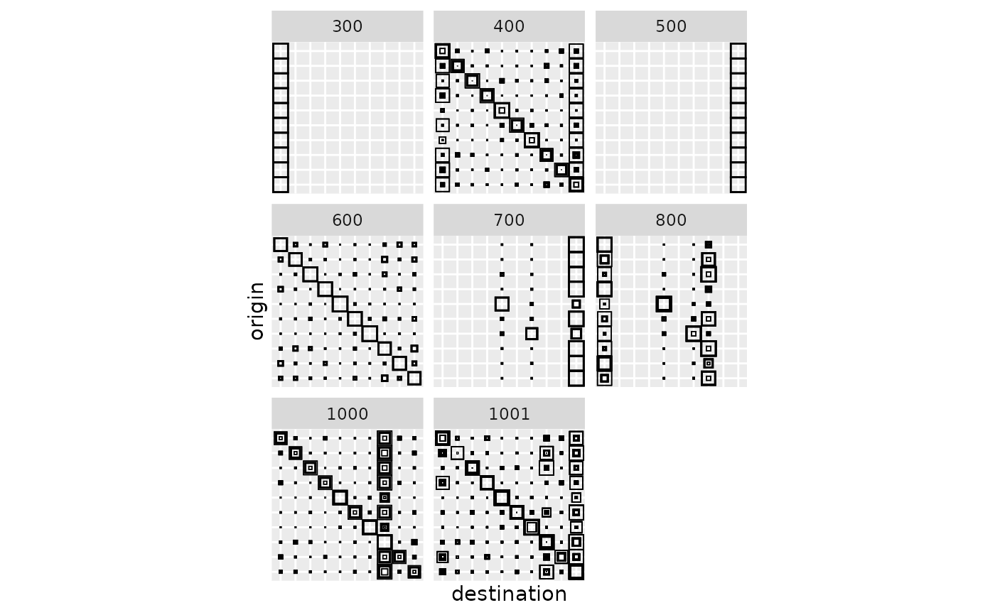
## group models by iteration number
grid_var_autoplot(all_flows_df, iterations)

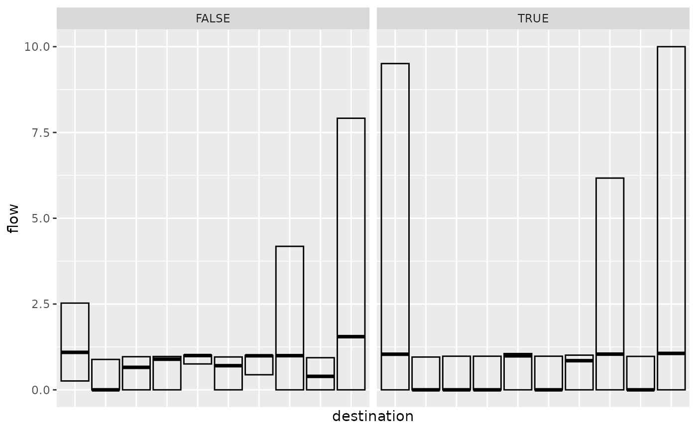
## or by convergence status (showing destination)
grid_var_autoplot(all_flows_df, converged,
  flows = "destination",
  with_names = TRUE
) + ggplot2::coord_flip()

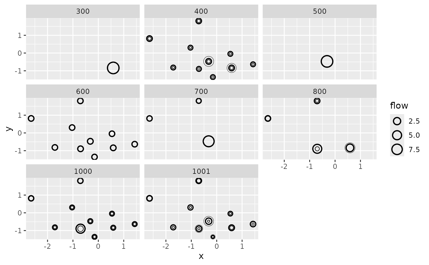
## using positions
grid_var_autoplot(all_flows_df, iterations,
  flows = "destination",
  with_positions = TRUE
) +
  ggplot2::scale_size_continuous(range = c(0, 3)) +
  ggplot2::coord_sf(crs = "epsg:4326")